A little pooling goes a long way for multi-vector representations

We’re releasing an early version of a simple token pooling trick for ColBERT. This allows for considerable memory&disk footprint reduction with very minimal retrieval performance degradation.

This blog post constitutes the first part of our exploration on this topic, with another, more in-depth one to follow.

Because retrieval can sometimes be a confusing topic, this blog post is structured in three main sections:

1. A key takeaway part, just summarising the findings in bullet-point forms.
2. A primer common deep learning based retrieval methods and ColBERT, explaining some core concepts as well as the issues they face.
3. Our token pooling trick, and how it works.

Key Takeaways

We experimented with various ways of improving the main weakness of ColBERT: vector count explosion (as each token requires storing a separate vector).

To do so, we introduce token pooling by clustering similar tokens within a given document and averaging (mean pooling) their representation. Our early results show that:

1. Token Pooling is a near-free lunch: a large reduction in vector count, and therefore memory use, can be achieved with only very minimal performance degradation, even when the vectors are then aggressively quantised.
2. We call the maximum number of tokens pooled together the Pool Factor: this is the number of tokens we will pool together, and therefore, the compression factor induced by pooling. We observe a sweet spot at pooling factors of 2&3 (with respectively no & little degradation), while it still holds strong at factor 4.
3. This simple method requires no model modification whatsoever, nor any complex processing, while greatly improving the scalability of easily updatable (“CRUD”) indexing methods, which are generally harder to use with ColBERT.

In fact, it is already live and ready to use in upstream ColBERT and will be supported in RAGatouille in the next few days.

We evaluate this approach on all small and medium-sized subsets of BEIR, the most commonly used set of retrieval evaluation benchmarks.

This shows a consistent pattern on all datasets, with one notable outlier where pooling tokens together actually considerably increases performance ¹.The graph below shows the relative performance of various pooling factors (where 100 is the retrieval performance without any pooling). After being pooled, the vectors are then quantised to 2-bits using the ColBERTv2 quantisation approach (read on to learn more about it!).

Multi-Vector Representations (ColBERT): How and Why?

Tip

If you’re interested in learning more about basic retrieval components, you should check out the talk I gave at Hamel Husain’s Mastering LLM course. Likewise, if you’re already familiar with basic retrieval components and ColBERT, you can skip to the next section.

Conventional Deep Retrieval

Traditionally, there are two main ways of using deep learning for retrieval:

Cross-Encoders

Cross-Encoders are also frequently called “rerankers”, although there are also other ways to rerank documents.

These models are functionally classifiers, and are passed both the query and a target document, therefore being aware of both at encoding time. They tend to produce the best retrieval performance, but they’re prohibitively expensive: the model must be ran on every single Query/Document pair in order to produce a ranking.

Bi-Encoders

Bi-Encoders are by far the most common approach to deep learning for retrieval. You’ve probably encountered them under a variety of names: dense embedders, single-vector representation, or, most commonly, just embeddings.

These models are what you’d most commonly think of as “embedding models”: they produce a single vector representation of a document by pooling the embeddings of the document’s tokens.

At query time, the query is also transformed into a single vector with the same model, and the list of relevant documents is produced by a simple cosine similarity nearest neighbour search between the query, and the previously encoded documents.

The shortcomings of this approach is a mirror of the cross-encoder’s shortcomings: bi-encoders are relatively computationally inexpensive, and very fast at scoring time, since cosine similarity is very easy to compute. However, your retrieval performance can suffer, especially on Out-Of-Domain data (i.e., yours): the training of these models teaches them to focus on learning to represent information that’d be relevant to their training queries, but that means it can very easily miss out on details and not represent the information you actually care about.

Basically, you’re asking the model to figure out a way to capture all the information within the document, in such that is can be retrieved by any relevant query, no matter the information it is looking for: this is a very hard task, especially when it needs to do so in just a single, relatively-small, fixed vector.

ColBERT and Multi-Vector Representations

Note

This is a very quick introduction to the underlying principles of ColBERT. If you want to find out more, I highly recommend reading Vespa’s Jo Kristian Bergum’s ColBERT blog post and the original ColBERT paper.

This is where multi-vector representation methods, generally also referred to as late interaction (see below) or, more simply, ColBERT, after the name of the main multi-vector model.

ColBERT tries to strike a middle ground. Effectively, it functions as a bi-encoder: all documents representations are pre-computed in isolation, with no query awareness.

However, the actual similarity computation occurs very late, and focuses on interactions between individual query and document tokens, rather than the full document. Hence the name for this method family: “late interaction”.

The process, with ColBERT, looks more like this:

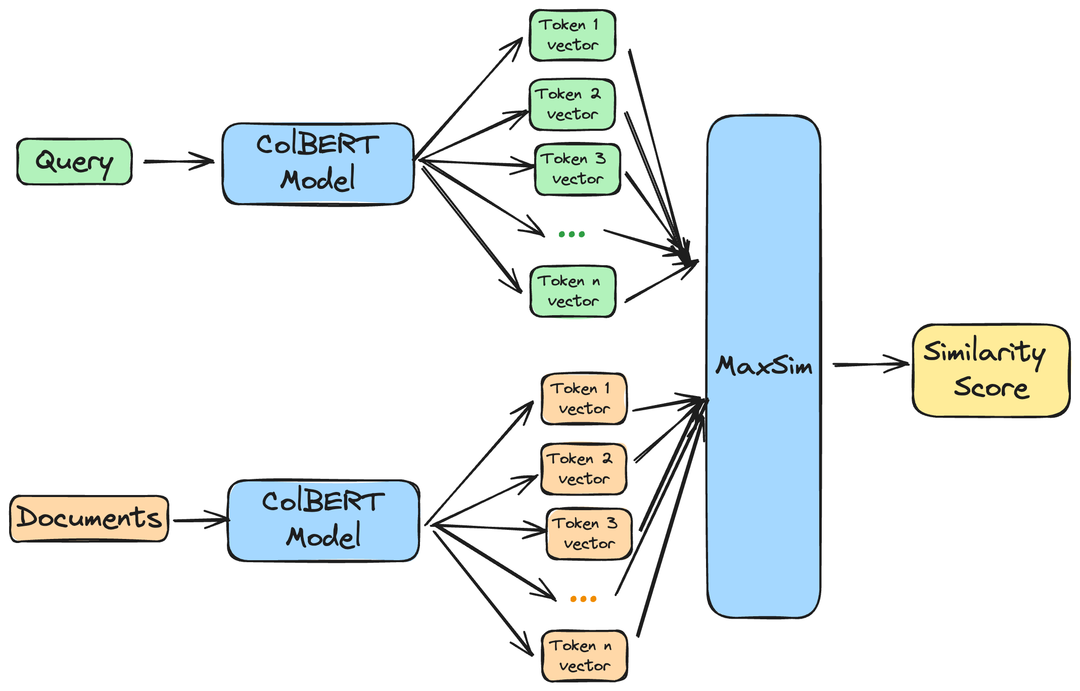
Essentially, ColBERT is a form of bi-encoder, with a different storage and scoring approach.

The representation for documents are still pre-computed, while queries are encoded at inference-time. However, rather than pooling these representations into a single vector early, we actually keep the token-level representations. At scoring time, we use the maxSim operator to compute the similarity between a given query and target documents.

maxSim sounds like another big word, but like most retrieval concepts, it’s actually pretty straightforward, for every query-document pair, we: - Compute the cosine similarity between each query token and all document tokens - Keep the highest, or maximum, of those similarity scores for each query token (hence **maxSim**, for maximum similarity) - Sum all those token-level maxSim scores together: this is the final similarity score of the query-document pair.

In practice, this allows for much greater generalisation potential: your models are no longer given the Sisyphean task of squeezing in all the relevant information (for both queries AND documents) into a single long vector!

Instead, “all” they have to do is create a (strong & contextualized) token-level representation that captures as much of the semantic meaning of a given token as possible. As text embedding is effectively a form of “meaning compression”, this is a much more relaxed effort: the model doesn’t need to learn to pool representations together, and gets a considerably larger space into which it must compress information, which raises the next point…

A tale of many floats: how to maintain efficiency with multi-vector representations

Tip

This section uses a lot of “retrieval jargon” about Indexes, which is unavoidable. Fully understanding what indexes are and what the various methods are isn’t necessary to understand the core idea of this section and fully defining them is out of scope of this already long article.

The main pre-requisite is simply understanding that an index is an efficient way to perform approximate rather than exact vector search. This means that search isn’t performed on all vectors but only on ones “likely” to help us return the relevant results. Exactly how this is done depends on the indexing methods, all of which have their own pros and cons.

The above sounds pretty perfect, doesn’t it? Of course, who doesn’t want finer-grained information about my documents that also generalises better? There must be a catch, right?

And there’s indeed a catch: it’s a lot less simple to work with multiple vectors. The two core reasons for this are very straightforward: having many more vectors means that storage and memory usage balloons up (problem 1), while also making it more complicated to efficiently search through them (problem 2).

While they sound similar, these two problems have different implications, so let’s quickly go through them:

Storage & Memory Efficiency

Note

This is a a very quick overview of the underlying mechanisms allowing ColBERT to scale. If you’re interested in the details of how quantisation is handled and so many vectors can be efficiently searched through, you should respectively look at the ColBERTv2 and PLAID papers.

This problem is obvious: when using a bert-base sized model to index a single document containing 300 tokens, we are getting:

• With a single-vector model: just one vector, containing 768 (bert-base’s embedding dimension) floating points number. Using 16-bit precision, this requires storing 1536bytes per document.
• With ColBERT: 300 (1 per token) vectors, each of them containing 768 floating points numbers, for a total of 230,400 floats. In 16-bit precision, this is 460,800bytes 🤯.

This is a gigantic increase in storage space: we’re effectively storing token_count times more data for each document!

This is obviously not something we want, nor is it scalable. Multiple methods are used to alleviate this:

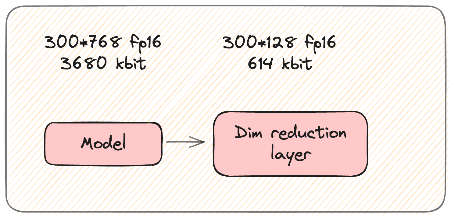
Dimensionality Reduction The first one is the most simple: Because of how much information fine-grained representations capture, we can safely reduce the dimensions of our output vectors. To do so, ColBERT uses a linear layer to cast its embedding dimensions from 768 to just 128.

This reduces the number of floats needed to store 300 tokens from from 230,400 (460,800 bytes) to 38,400 (76,800 bytes). This is still considerably more than 768, but is already an order of magnitude lower than our raw output – phew!

This is what the pipeline looks like at this stage:

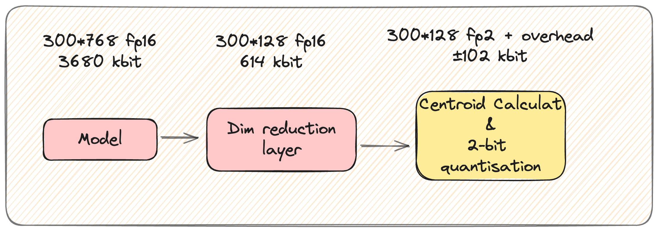
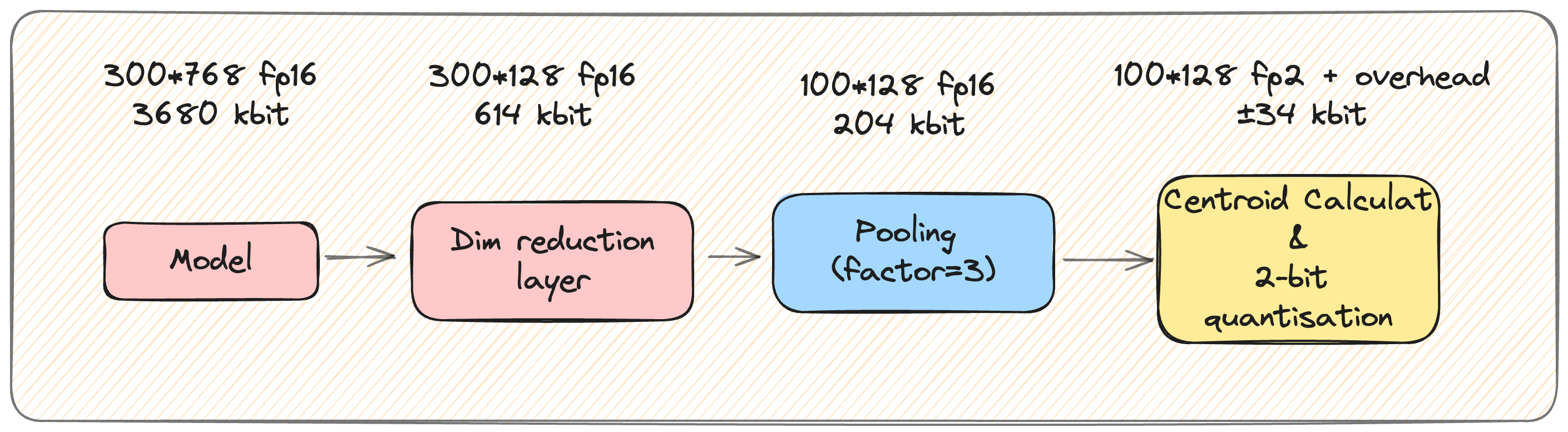
Extreme Quantization ColBERTv2 goes further and introduces another approach on top of reducing the per-vector dimensions: extreme quantization.

Essentially, the team behind ColBERT refines their approach, and finds that high precision isn’t necessary for multi-vector representation, in large part because tokens tend to naturally cluster into semantic regions in the cluster-space.

Thanks to this phenomenon, it becomes possible to delegate much of the useful information to the centroids of these clusters, while aggressively compressing each individual token-level vector to just 2 bits, while losing very little retrieval performance. This is fundamentally a form of IVF-PQ (Inverted File Index-Product Quantisation) indexing, a very popular quantisation-powered indexing method, which you can read more about in this excellent introducton by LanceDB.

It’s worth noting that this isn’t quite the full 8-fold storage reduction you’d expect from 2-bit compression, as there’s overhead introduced by the necessity of storing additional information to accurately map each token to its centroid. However, this method still reduces storage requirements by an impressive factor of 6, the resulting index requiring only around ~16.7% of the pre-compression storage space: this brings the footprint of a 300 token document down to just ~12,800bytes.

With this step, this is what the pipeline now looks like:

How to efficiently search through so many vectors?

While compressing vectors is a step in the right direction, it doesn’t solve the elephant in the room: the sheer computational cost of searching through millions of vectors.

Candidate Generation: Minimising the impact of token-level scoring

While you can easily search through thousands-to-tens-of-thousands single-vector representations in memory (aka brute-force search), doing so with ColBERT will result in noticeable slowdowns after just a few hundred documents.

This makes sense: we are searching through a lot more vectors, and performing a very large number of comparisons. This is partially due to how maxSim works: not only are documents represented by many more vectors, but we must also compute similarities for every query token, rather than just once for the whole query.

In retrieval, it’s common to build an index to perform approximate search very efficiently. This is for example what is done by methods such as ColBERTv2+PLAID’s IVFPQ-like approach, mentioned above. Indexes are particularly powerful: through efficient searching methods and at a low cost to retrieval accuracy ², they’re able to retrieve results in a handful of milliseconds.

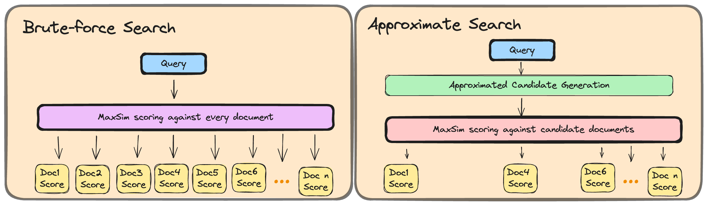
All ColBERT indexing methods partially address this problem by introducing a candidate generation step: effectively, during this stage, we use a form of approximate search to pre-retrieve up to k passages, and maxSim will only be ran on those candidates. This greatly reduces the number of similarity computations we need to compute.

As a result, index-based approximate-search is generally used as ColBERT’s candidate generation step. Doing so allows us to fully process queries in just a few dozen milliseconds, even with millions of documents.

An Unsolved Problem: Index-Building and CRUD capabilities

However, while these methods address the issue of slow scoring, it doesn’t address another one: building indices to generate these candidates is particularly costly when storing so many vectors.

Think about it from our previous example, where our documents contain 300 tokens: To store just 1000 documents with single-vector representations, you only need to index 1000 vectors, whereas ColBERT requires indexing 300*1000=300 000 vectors!

There are two main costs to this. The first one is fairly straightforward: for all indexing methods, building a ColBERT index takes longer than building a traditional index. This is a one-time cost at indexing time.

The second and considerably more important downside is more subtle. Storing so many vectors requires complex index mapping, and the way this manifests is in an important trade-off between the two most used indexing methods:

• IVF-PQ-style indexing (ColBERTv2’s default, PLAID) can scale to millions and millions of documents, but sacrifices CRUD capabilities: adding documents is extremely slow (to the point rebuilding the index makes more sense in many cases), and removing documents is largely unsupported.

• HNSW-style indexing, another very common indexing method, retains CRUD capabilities, but scales poorly: as more documents are added, the overhead for each new addition increases noticeably. Additionally, extreme quantisation isn’t as easy to use with this kind of index and would result in larger performance degradations: this means all widely used HNSW implementations are at risk of hitting memory allocation limits when building “larger” (>10,000s of documents) indexes.

These problems are tough to address, and there currently doesn’t exist a silver bullet solution. However, we’re finally getting to the meat of this blog post: a simple solution to greatly reduce the disk, memory and vector-count footprint of ColBERT.

Token Pooling

And after this long introduction, we’re getting to our actual contribution: the early release of Token Pooling for ColBERT.

The Why and How of Vector Count Reduction

Reducing vector count serves two important goals, which are direct answers to the two problems highlighted above. These goals are:

• Lowering the memory&disk usage: This can further alleviate scaling issues, and reduce hardware requirements for larger indexes.

• Considerably increasing the scalability of CRUD-friendly methods, such as brute-force search or HNSW-indexing the vector count. This is very important to everyday use: many document collections are fairly small and specialised, and removing the need for heavy-duty infrastructure to handle them is a great accessibility improvement.

This is by no means a new area of research. There is existing work exploring token pruning, which consists in removing certain tokens. Different approaches exist, but the challenge of identifying which tokens to remove is always complex, especially as “irrelevant tokens” for certain queries might turn out to be very useful for others.

Moreover, many of these vector count reduction approaches rely on methods which require model changes: for example, ColBERTer ³ attempts to reduce the storage cost of ColBERT by a mix of techniques, the main one being the use of whole-word representations. However, this requires a specifically trained model and a considerably more complex pipeline.

Our goal with this work is to introduce a simple method, that works out-of-the-box with any existing multi-vector representation model. We do so by using the same concept used to create single-vector representations: pooling.

Why would we pool tokens?

Tip

Pooling token representations is a simple and well-explored concept in NLP: it’s effectively just the act of merging multiple vectors into a single one.

There are multiple ways to pool vectors, but one of the most common one is mean pooling: this means that the final vector is the average of the vectors pooled together to create it.

The core idea of ColBERT, funnily enough, is to go against pooling as it’s most commonly performed: into a single-vector. On the other hand, we believe that introducing a small degree of pooling could go a long way!

The intuition as to why goes back to tf-idf: not all tokens are created equal. More recently the XTR⁴ paper explores this same idea with ColBERT, and shows strong results with an alternative scoring approach only focusing on a subset of tokens.

To put it simply, we start off the assumption that within a given document, the importance of the information conveyed by various tokens is wildly varied: some tokens are highly informative, some are highly uninformative, and the rest sit in the middle.

Moreover, we also assume that for documents focusing on a low number of topics, a lot of the tokens are likely to carry somewhat redundant semantic information, meaning keeping all of them is likely not useful.

Finally, there’s a recurring problem that is important to keep in mind when attempting to reduce vector count. While not all tokens are useful to answer a given query, we have no way of knowing ahead of time which tokens are going to be unnecessary. Therefore, vector count reduction methods must be wary of suppressing information rather than simply compressing it.

How does it work?

Keeping in mind all of the above, we decide to perform token pooling at indexing time. We want to base our pooling based on how redundant tokens are likely to be.

To do so, we devised three ways of pooling tokens:

• “You shall know a word by the company it keeps”⁵: The most naive method imaginable, pooling sequential tokens together, via a sliding window.

• Two methods relying on the cosine similarity of individual token representations:

  • A simple, k-means based method.
  • A hierarchical clustering approach.

We will go more in-depth about all three methods and their results in the future. For now, our early experiments showed that hierarchical clustering is, in all cases, the superior approach, and is thus the one we’ve chosen to focus on at this point.

The pooling process is very simple, and lives within a couple dozens lines of code:

Show the code

def pool_embeddings_hierarchical(
    p_embeddings,
    token_lengths,
    pool_factor,
    protected_tokens: int = 1,
):
    device = torch.device("cuda" if torch.cuda.is_available() else "cpu")
    p_embeddings = p_embeddings.to(device)
    pooled_embeddings = []
    pooled_token_lengths = []
    start_idx = 0

    for token_length in tqdm(token_lengths, desc="Pooling tokens"):
        # Get the embeddings for the current passage
        passage_embeddings = p_embeddings[start_idx : start_idx + token_length]

        # Remove the tokens at protected_tokens indices
        protected_embeddings = passage_embeddings[:protected_tokens]
        passage_embeddings = passage_embeddings[protected_tokens:]

        # Cosine similarity computation (vector are already normalized)
        similarities = torch.mm(passage_embeddings, passage_embeddings.t())

        # Convert similarities to a distance for better ward compatibility
        similarities = 1 - similarities.cpu().numpy()

        # Create hierarchical clusters using ward's method
        Z = linkage(similarities, metric="euclidean", method="ward")
        # Determine the number of clusters we want in the end based on the pool factor
        max_clusters = (
            token_length // pool_factor if token_length // pool_factor > 0 else 1
        )
        cluster_labels = fcluster(Z, t=max_clusters, criterion="maxclust")

        # Pool embeddings within each cluster
        for cluster_id in range(1, max_clusters + 1):
            cluster_indices = torch.where(
                torch.tensor(cluster_labels == cluster_id, device=device)
            )[0]
            if cluster_indices.numel() > 0:
                pooled_embedding = passage_embeddings[cluster_indices].mean(dim=0)
                pooled_embeddings.append(pooled_embedding)

        # Re-add the protected tokens to pooled_embeddings
        pooled_embeddings.extend(protected_embeddings)

        # Store the length of the pooled tokens (number of total tokens - number of tokens from previous passages)
        pooled_token_lengths.append(len(pooled_embeddings) - sum(pooled_token_lengths))
        start_idx += token_length

    pooled_embeddings = torch.stack(pooled_embeddings)
    return pooled_embeddings, pooled_token_lengths

Effectively, we must first define a Pool Factor: this is the factor by which we will reduce the total token count. For example, this means that, for a Pool Factor of 3, we will pool tokens into total_tokens_count/3 clusters, reducing the total number of vectors by 66.7%.

Note

Please note that our best performing approach, which we’re releasing today, is using hierarchical clustering rather than k-means.

This means that the Pool Factor works slightly differently than you’d expect: there is no guarantee that each individual cluster will contain Pool Factor tokens, only that there will be total_token_count/Pool Factor clusters in the end. In early experiments, we have observed that despite this, the tokens seem to be very evenly distributed between clusters, but this is not guaranteed.

The process is then conducted in a few step. For each document, we:

• Compute the cosine similarity between all of its individual token representations
• (Optionally) Protect certain tokens, such as the [CLS] (which is already a pooled representation) and [D] (which lets the model know it’s encoding a document) tokens
• Create total_token_count/Pool_Factor clusters, built by maximising the cosine similarity calculated above.
• Iterate through tokens and add them to the cluster to which they’re most similar.
• Mean pool the representation of tokens within a given cluster into a single vector.

And that’s pretty much it! Each cluster ends up represented by a single token, created from the average values of the tokens which it contained. This is how the PLAID pipeline highlighted above looks like with the addition of the Pooling step:

How *well* does it work?

The answer to this question is surprisingly well. Our initial expectation was that the results would be interesting, but would only serve to support further exploration. However, in practice, we found that we were able to achieve a sizeable reduction of stored vector count while having only a minimal impact on retrieval accuracy. We ran our early experiments on a set of small datasets from BEIR, using uncompressed (16-bit) vector representations. The graph below shows our results:

To evaluate our results, we measure the impact on retrieval performance: we define the unpooled results as our reference point, i.e. 100%, and evaluate the impact of pooling.

Immediately, we can see that there’s a noticeable drop with Pool Factors of 4 and above. At a factor 4, meaning that we reduce the vector count to 25% of the original total, the average retrieval performance decreases to 97% of the unpooled approach, and drops further from that point on.

However, low pool factors fare remarkably well: Pooling by a factor 2 achieves a 50% vector count reduction while actually achieving a small improvement, reaching 100.6% retrieval performance on average. Increasing the factor to 3 gets us to a 66% reduction, while still reaching 99% of the original scores.

These sizeable reductions have a noticeable real-world impact. On an 8GB RAM test machine, we were unable to create an uncompressed index for TREC-Covid, reaching memory limits when building the index. However, this became possible with a pool factor of just 2!

What about Quantisation?

In the previous section, we introduced the 2-bit quantisation approach commonly used with ColBERT. Naturally, this raises the question of whether or not this pooling method is robust to being aggressively quantised.

We evaluate our method with 2-bit quantisation on the same datasets as above, as well as two larger BEIR datasets: Webis-Touché and TREC-COVID.

The table below presents the results on all 6 evaluation sets, as well as their average with and without the two outliers:

The immediate elephant in the room is Webis-Touché: not only does performance not decrease, but it increases by up to 40%, with the boost growing with the Pool Factor. \ There’s another outlier, although much less drastic: fiqa, where, on the other hand, the performance decreases considerably quicker than on others.

We haven’t yet studied the mechanism enough to understand why this different behaviour occurs (although, Touché is known for often yielding different results from other datasets⁶), but we are very much planning on exploring this in the coming weeks!

Overall, we do still observe a pattern that is very similar to the one without quantisation: even when accounting for fiqa, the highest performance drop for a pool factor of 2 is below 3%.

Interestingly, for TREC-Covid, the largest scale commonly used dataset that we included in our evaluations, the performance is remarkably stable: between pooling factors of 2 to 6, the performance of pooling remains slightly above the one of unpooled vectors.

How to use this?

It’s already implemented in upstream ColBERT, with RAGatouille support coming in the next few days!

Using it is pretty simple: it must simply be enabled it at indexing time, so we can compress document prior to indexing them. We’ve implemented the feature using ColBERT’s existing configuration system, which means that all you need to do is to set a pool_factor higher than 1 in your config.

For example, if you wanted to modify the ColBERT’s README example to use pooling, the only change required would be the extra config argument here:

from colbert.infra import Run, RunConfig, ColBERTConfig
from colbert import Indexer

if __name__=='__main__':
    with Run().context(RunConfig(nranks=1, experiment="msmarco")):

        config = ColBERTConfig(
            nbits=2,
            root="/path/to/experiments",
            pool_factor=2, # This is the key line to add! Tweak the factor as you see fit!
        )
        indexer = Indexer(checkpoint="/path/to/checkpoint", config=config)
        indexer.index(name="msmarco.nbits=2", collection="/path/to/MSMARCO/collection.tsv")

And that’s it!

What’s next?

This post doesn’t have a proper conclusion, since we started the post with it (🔗)! Instead, we’ll end on this quick message about future plans :)

Bear in mind: this is an early release, and we’re actively looking more into it! While we get very strong results, this is just a first step. We’re currently focusing on evaluating the various methods on a broad range of datasets, and trying to understand why this method works so well, as well as the differences we observe between different datasets. Following this, we intend to further delve™️ onto more ways of making multi-vector retrieval more efficient. Stay tuned for the upcoming posts (and papers 👀?)!

Footnotes

1. We don’t have an explanation for this yet, although it is generally considered to be a “strange” dataset, which has been explored in a very recent SIGIR24 paper by Thakur et al.. We do plan on exploring the reasons why pooling works so well in upcoming work, so stay tuned!

2. This cost is extremely low for ColBERT, as the candidate generation step will retrieve candidate documents for each query token, further minimising the likelihood that the approximate search has missed relevant documents. This is due to the fact that a relevant document is very unlikely to not have any of its tokens belong to the top matches of at least one query token.

3. Introducing Neural Bag of Whole-Words with ColBERTer: Contextualized Late Interactions using Enhanced Reduction (2022), Hofstätter et al.

4. Rethinking the Role of Token Retrieval in Multi-Vector Retrieval (2023), Lee et al.

5. You’ll have recognised what’s potentially the most used quote in NLP, from John Rupert Firth’s 1957 A Synopsis of Linguistic Theory

6. We don’t have an explanation for this yet, although it is generally considered to be a “strange” dataset, which has been explored in a very recent SIGIR24 paper by Thakur et al.. We do plan on exploring the reasons why pooling works so well in upcoming work, so stay tuned!